7 Visualization and reporting
ROI analysis
See also: Planning 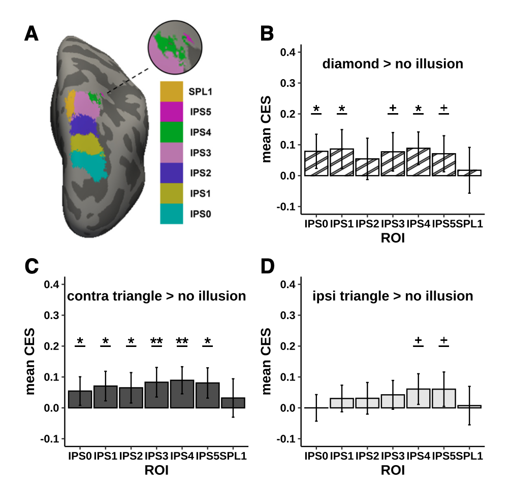
If you were planning a ROI analysis, you will typically have one value per ROI, subject and condition. You can report descriptive statistics graphically using your favourite approach (violin plots, bar plots, boxplots, etc.).
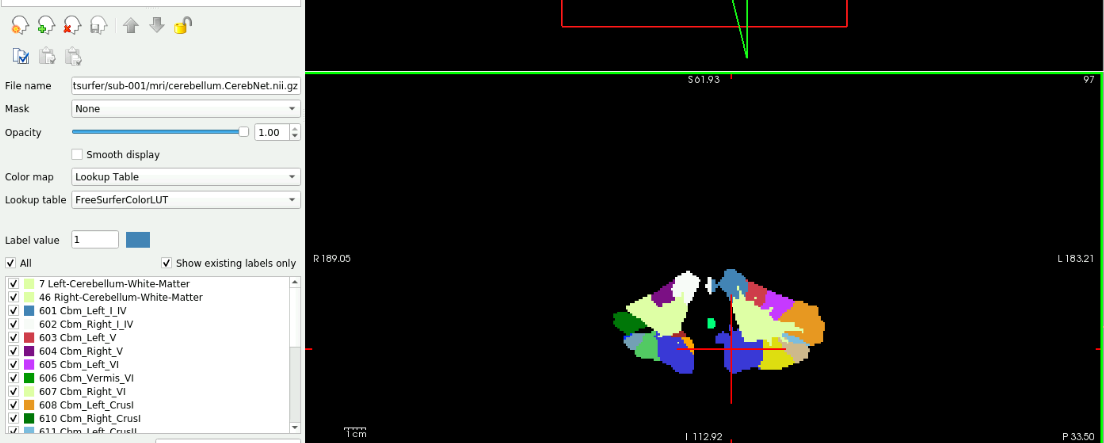
Usually we also visualize ROIs at their locations.
Example
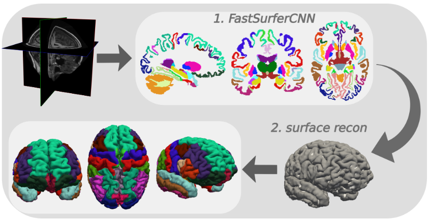
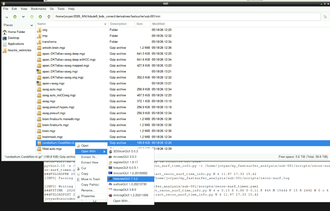
Run the segmentation
Deep-MI/FastSurfer: PyTorch implementation of FastSurferCNN
# create the directory
mkdir /home/jovyan/2026_ANI/lobule9_bids_correct/derivatives/fastsurfer

# run the fastsurfer as a singularity container
singularity exec --nv \
                 --no-mount home,cwd -e \
                 -B $HOME/2026_ANI/lobule9_bids_correct:$HOME/my_mri_data \
                 -B $HOME/2026_ANI/lobule9_bids_correct/derivatives/fastsurfer:$HOME/my_fastsurfer_analysis \
                 -B $HOME/license.txt:$HOME/my_fs_license.txt \
                 /shared/singularity/fastsurfer-gpu.sif \
                   /fastsurfer/run_fastsurfer.sh \
                     --fs_license $HOME/my_fs_license.txt \
                     --t1 $HOME/my_mri_data/sub-001/ses-1/anat/sub-001_ses-1_acq-mprage_T1w.nii.gz \
                     --sid sub-001 --sd $HOME/my_fastsurfer_analysis \
                     --3T \
                     --threads 4 \
                     --seg_only
View output
Multiple comparison correction
Reminder: group analysis
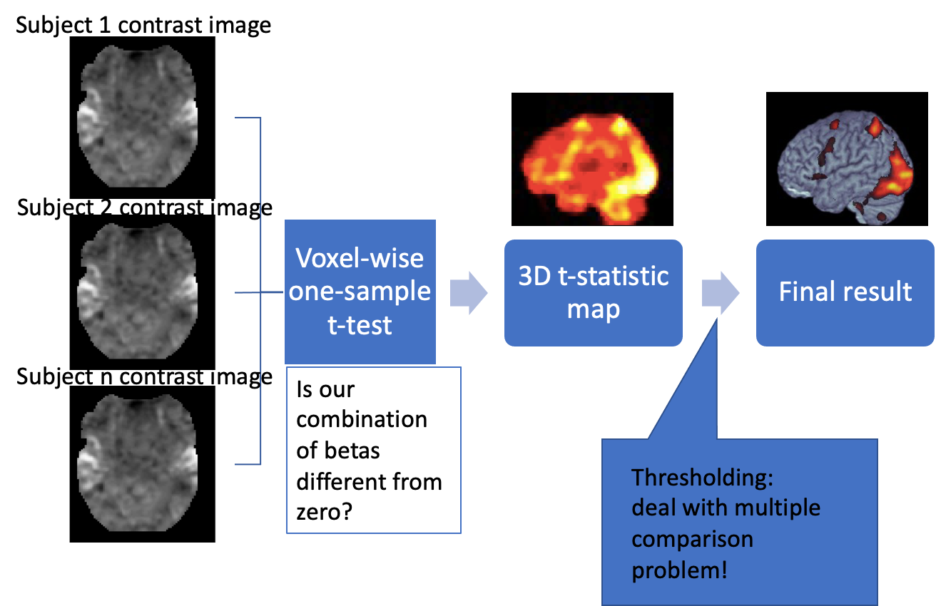
Family-wise error rate
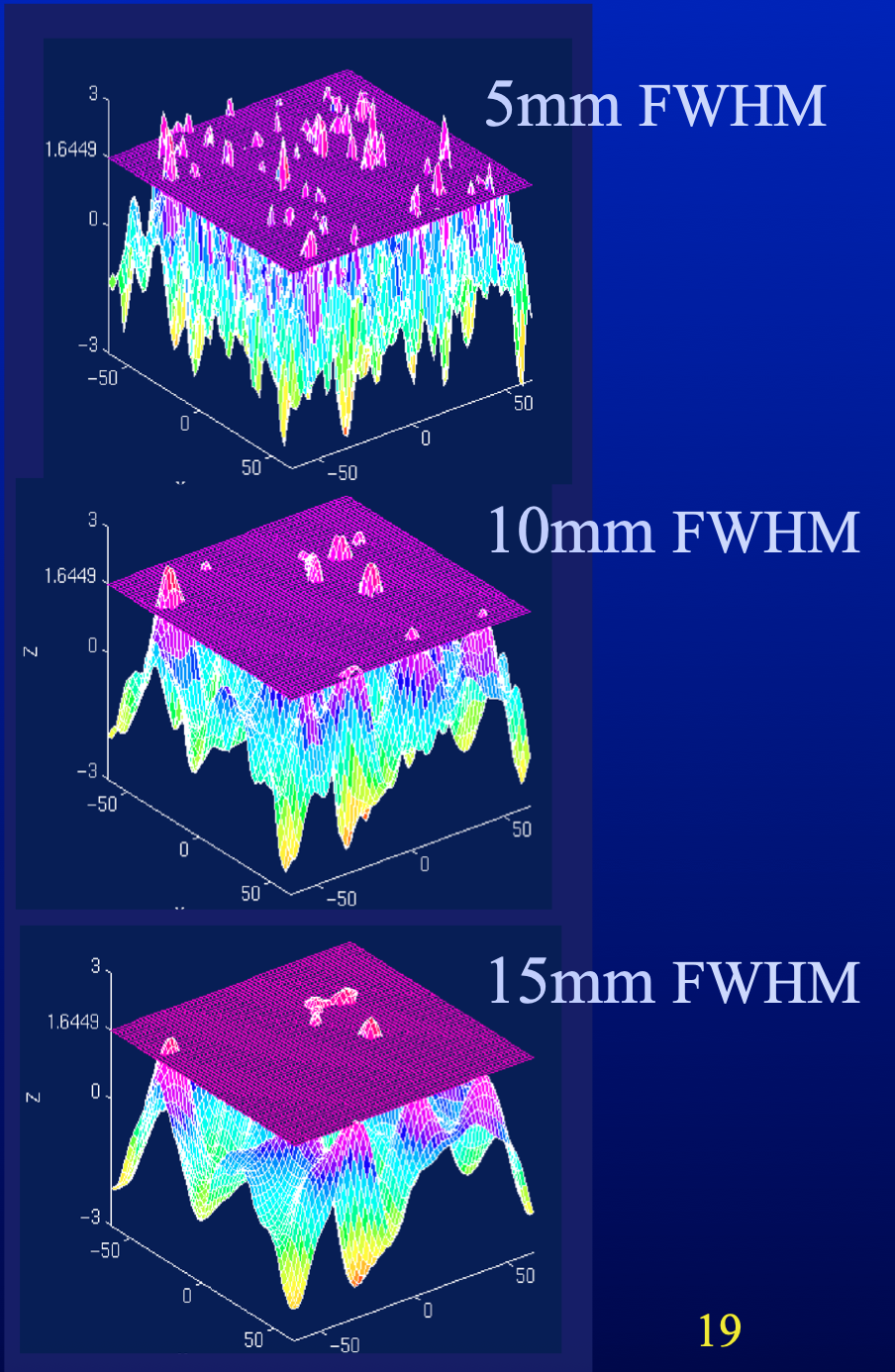
If the data is not smoothed, equivalent to Bonferroni correction
Other correction types
- Cluster threshold
- False discovery rate
- Cluster-level inference
Uncorrected
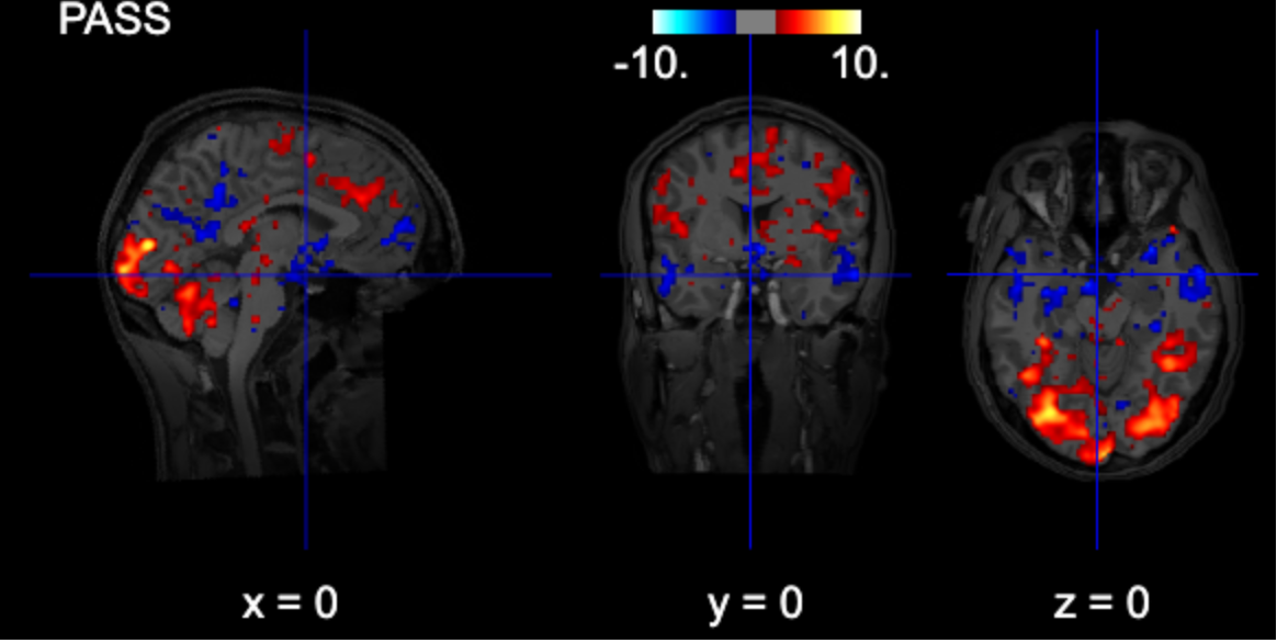
# interactive plot (you can browse the activations)
from nilearn import plotting

# Use subject's anatomy as background
bg_img = '/home/jovyan/gambling/bids/derivatives/fmriprep/sub-001/ses-1/anat/sub-001_ses-1_acq-mprage_desc-preproc_T1w.nii.gz'
plotting.view_img(zmap, threshold=1.96, vmax=10,
    bg_img=bg_img,
    cut_coords=[0, 0, 0],
    width_view=600,
    title=contrast_string)
Cluster-thresholded
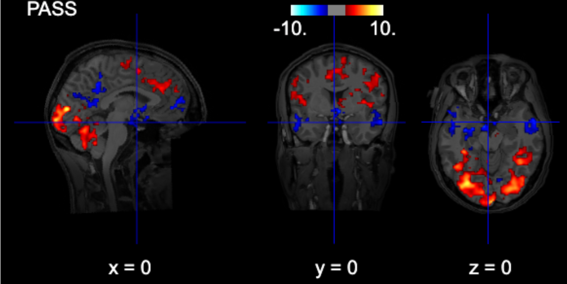
from nilearn.glm import threshold_stats_img

# note: fpr with alpha=0.05 is the same as uncorrected z>=1.96 (p<0.05)
thresholded_map1, threshold1 = threshold_stats_img(
    zmap,
    alpha=0.05,
    height_control="fpr",
    cluster_threshold = 100,
    two_sided=True,
)

# Use subject's anatomy as background
bg_img = '/home/jovyan/gambling/bids/derivatives/fmriprep/sub-001/ses-1/anat/sub-001_ses-1_acq-mprage_desc-preproc_T1w.nii.gz'
plotting.view_img(thresholded_map1, threshold=threshold1, vmax=10,
    bg_img=bg_img,
    cut_coords=[0, 0, 0],
    width_view=600,
    title=contrast_string)
FDR-thresholded
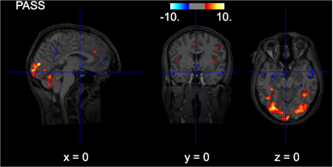
from nilearn.glm import threshold_stats_img

thresholded_map1, threshold1 = threshold_stats_img(
    zmap,
    alpha=0.05,
    height_control="fdr",
    two_sided=True,
)

# Use subject's anatomy as background
bg_img = '/home/jovyan/gambling/bids/derivatives/fmriprep/sub-001/ses-1/anat/sub-001_ses-1_acq-mprage_desc-preproc_T1w.nii.gz'
plotting.view_img(thresholded_map1, threshold=threshold1, vmax=10,
    bg_img=bg_img,
    cut_coords=[0, 0, 0],
    width_view=600,
    title=contrast_string)
FWE-thresholded
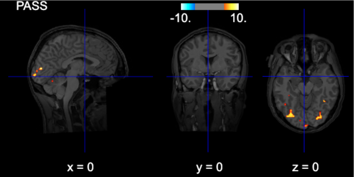
from nilearn.glm import threshold_stats_img

thresholded_map1, threshold1 = threshold_stats_img(
    zmap,
    alpha=0.05,
    height_control="bonferroni",
    two_sided=True,
)

# Use subject's anatomy as background
bg_img = '/home/jovyan/gambling/bids/derivatives/fmriprep/sub-001/ses-1/anat/sub-001_ses-1_acq-mprage_desc-preproc_T1w.nii.gz'
plotting.view_img(thresholded_map1, threshold=threshold1, vmax=10,
    bg_img=bg_img,
    cut_coords=[0, 0, 0],
    width_view=600,
    title=contrast_string)
Non-parametric inference
Permutation-based inference
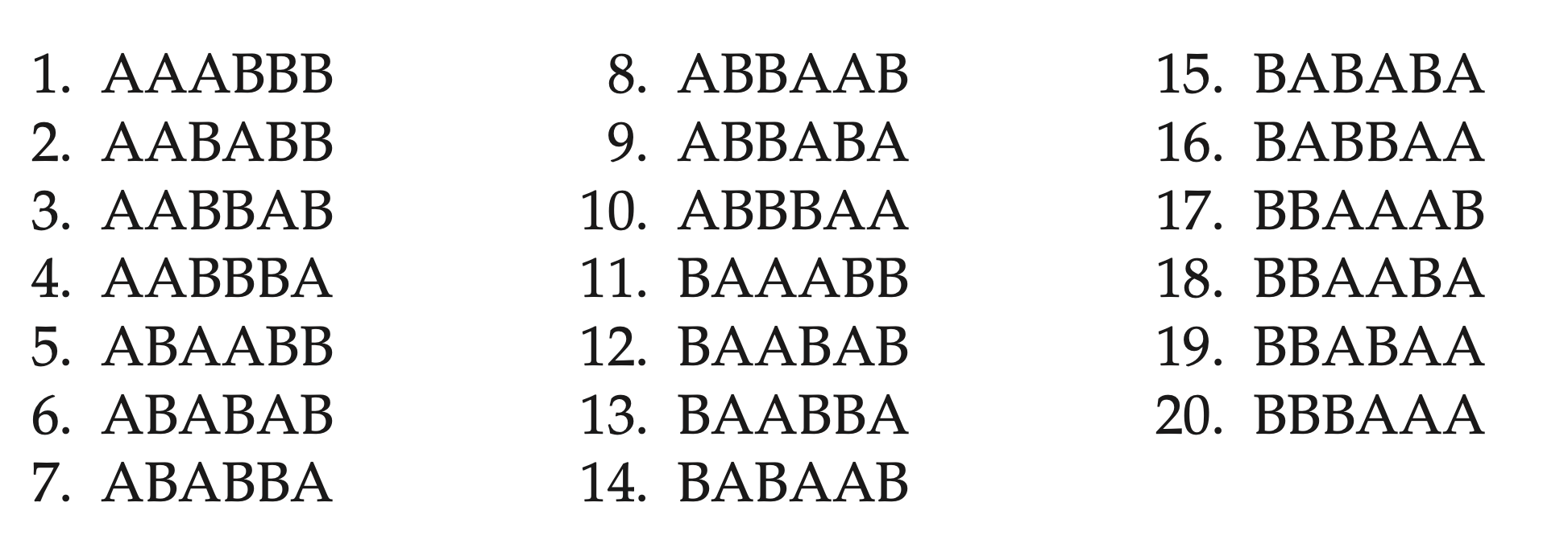
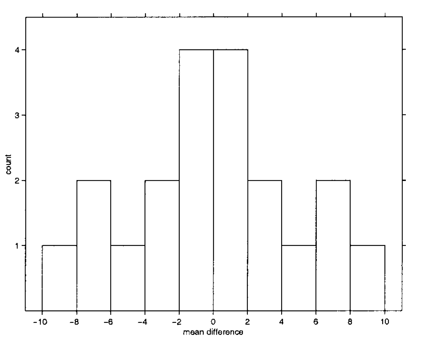
An example difference between conditions A and B. The labels of each trial are permuted and each time a test statistic (in this example mean difference) is computed. The empirical likelihood to observe a specific value is derived.
For the multiple comparison case, we use the same logic, but instead of single voxel we consider the maximum of each statistical map.
Result reporting
Whole-brain analysis
P-value threshold, MC correction method
All clusters with
size
peak statistic value
MNI coordinates
anatomical area (see atlasreader and the associated notebook)
Region-of-interest analysis
- MCC for the number of areas examined