4 Preprocessing

of an fMRI dataset

Preprocessing of fMRI data is intended for reducing the impact of MR artifacts and enhancing the data quality.

In principle, if the data quality is good and the subject did not move (which is the case for our experiment) preprocessing should not even be necessary. Nevertheless, this is a tradition that goes back to the 1990-es, and researchers mostly stick to it.

The maths behind these steps is oftentimes complicated, and most fMRI ‘users’ do not understand it. Our fMRI lab even offers to provide you with preprocessed data. I think it is important to know what you are doing, so we will go through basic preprocessing steps today.

Reminder: a typical experiment

To help us better understand the preprocessing steps, let’s remind ourselves about a typical fMRI experiment with a flickering checkerboard. In this experiment, we want to find out which brain areas are active when subjects view a flickering checkerboard compared to when they view a gray background. We have shown to every volunteer a checkerboard for e.g. 20 second interleaved with a 20 s rest, and we will measure a whole brain volume every 2 seconds, for e.g. to minutes or so.

Matlab code to generate stimulus, BOLD and shifted BOLD X = [1 1 1 1 1 1 1 1 0 0 0 0 0 0 0 0 1 1 1 1 1 1 1 1 0 0 0 0 0 0 0 0 1 1 1 1 1 1 1 1 0 0 0 0 0 0 0 0]; bf = spm_get_bf; % indicated a tr of 2.5 Y = conv(X,bf.bf); Ye = Y+randn(size(Y)).*0.2;

4D functional dataset

And, in a functional experiment we usually measure brain activity across the whole volume over extended perionds of time, so it is comfortable to think about each functional dataset that we acquire as a 4D dataset, which consists of 3D brain volumes and time as a 4th dimension.

Major software

Since 1994 http://www.fil.ion.ucl.ac.uk/spm/

Since 1994 http://afni.nimh.nih.gov/afni/

Since 2000 http://fsl.fmrib.ox.ac.uk/fsl/fslwiki/

Preprocessing used to be integrated into the software used for the actual analysis. And there are many software for this. On this slide I just put a few of them. Each of them has a slightly different phylosophy behind it, but all of them do roughly the same thing, so at the end it should not matter much which of them you use.

One of the oldest ones are:

SPM – statistical parameteric mapping from UCL. It is a free MATLAB-based toolbox. However, it depends on the MATLAB licence, and has not been updated for a long time. The new update just came out which spans the gab from 2012 to 2025 (Tierney et al. 2025).
AFNI - from NIH
FSL from Oxford – a set of linux tools, also free and independent of MATLAB, which is an advantage, but requires Linux.
FreeSurfer/FSFAST form the Martinos center - it is Linux based, and was originally conceived as a tool for structural data analysis, but has an fMRI module

Historical software

broccolli, that can utilize GPU computing and can process the same dataset n times faster

With the awareness of open science, and with the trend towards reproducibility and transparency, and with the release of fMRIprep software, the preprocessing got detached from the actual data analysis.

fMRIprep

Image source (Esteban et al. 2018)

fMRIprep has evolved to combine best practices in fmri preprocessing and also to unify and standardize analysis steps. It is currently dominating the field and is the state-of-the-art way to do preprocessing.

All the steps we will talk about are implemented in fMRIprep.

Anatomical preprocessing

Bias field correction

# gambling: view the before and after images by typing
ml freesurfer
freeview \
/home/jovyan/gambling/bids/sub-001/ses-1/anat/sub-001_ses-1_acq-mprage_T1w.nii.gz \
/home/jovyan/gambling/bids/derivatives/fmriprep/sub-001/ses-1/anat/sub-001_ses-1_acq-mprage_desc-preproc_T1w.nii.gz

Varying intensities across the image will confuse subsequent steps.

Surface reconstruction

# gambling: view the reconstructed surfaces by typing
ml freesurfer
freeview \
/home/jovyan/gambling/bids/derivatives/fmriprep/sourcedata/freesurfer/sub-001/mri/orig.mgz \
-f /home/jovyan/gambling/bids/derivatives/fmriprep/sourcedata/freesurfer/sub-001/surf/*h.white \
/home/jovyan/gambling/bids/derivatives/fmriprep/sourcedata/freesurfer/sub-001/surf/*h.pial

Relatively lengthy (some hours) multistage fully automatic process

Normalization

Will be discussed in the section on functional data

Functional preprocessing

# gambling: compare before and after my typing
ml freesurfer
freeview \
/home/jovyan/gambling/bids/sub-001/ses-1/func/sub-001_ses-1_task-gambling_acq-Fs2_run-1_bold.nii.gz \
/home/jovyan/gambling/bids/derivatives/fmriprep/sub-001/ses-1/func/sub-001_ses-1_task-gambling_acq-Fs2_run-1_space-T1w_desc-preproc_bold.nii.gz

As I already mentioned, preprocessing is not strictly necessary, especially with modern 3 Tesla scanners and compliant subjects. It is more important for high-field scanners which contain stronger artifacts, subjects that move a lot, or in spatial scenarios where we want to detect small effects and do not want to make sure we get rid of noise as much as we can.

The curious among you can try performing statistics with and without preprocessing and compare as a bonus task.

Here are the examples of functional and anatomical data before and after preprocessing. Do we see any difference? Not always. Especially for the functional data, the differences are seen over time and not so much over space.

Non-steady-state artifacts

Aka T1 equilibration artifacts

# gambling
file:///home/jovyan/gambling/bids/derivatives/mriqc/sub-001/figures/sub-001_ses-1_task-gambling_acq-Fs2_run-1_desc-carpet_bold.svg

I could not really spot this artifact in the scans we acquired to show you. This may be due to two facts:

Our scanner is quite good and modern, so these artifacts are minimal
The scanning protocol automatically acquires two volumes with those artifacts that are discarded

Perhaps these large intensity fluctuations on the left (in the beginning) in this carpet plot reflect this.

But non-steady-state artifacts are actually the reason why I asked to include a 10-second period where nothing is happening into the experimental paradigm. Non-steady-state volumes should not overlap with the actual experimental paradigm. In the past, we waited for 4-5 volumes before the actual paradigm started, and then discarded these volumes during preprocessing, so that data and paradigm are temporally aligned. But the non-steady-state volumes have an advantage of having good gray-white matter contrast. Therefore, fMRIprep tries to automatically identify them for each run and use them to produce a “reference scan”, which is used in the subsequent steps.

Motion correction

Purpose: compensate for subject movement

One of the first preprocessign steps is motion correction. Why do we need motion correction? During the fMRI experiment the subject is supposed to lay still inside the scanner, and they usually do so. However, even your best volunteer won’t be perfect. And in fMRI, even a few millimeters screw up your experiment. Here is an example. Let’s say we are measuring a voxel located on the left hemisphere, and the subject suddenly moved. As a result, the same voxel will be now recording activity from the empty space between the hemispheres, or even form the opposite hemisphere.

Motion correction

6 parameter “rigid body” transform

Usually, motion is much smaller, but we still want to correct it. How do we do this? Luckily there are special algorithms that can estimate the amount of motion from one volume to the next. This is usually done using 6 degrees of freedom: translation in x, y, and z and rotation in x, y, and z. This is called the “rigid body transform”, because you do not change the size and shape of the volume, but simply rotate it in space. After the amount of motion has been calculated, it can be applied to every image to align it back to the necessary position.

Plot motion parameters

Slice-time correction

Purpose: compensate for the lag in slice acquisition

The next preprocessing step is slice-time correction. What is slice time correction and why do we need it? Remember that typically a functional volume is acquired not all at once, but slice-by-slice, as illustrated here. There are different ways in which the scanner can acquire the slices: it can bie botton-to top (ascending), decending, interleaved. There are also more complex slice acquisition patterns. Remember that the time it takes to acquire one volume is relatively long, in this our example it is 2 seconds. Let’s say a stimulus activates two areas, here and here in the same manner. If we acquire the slices in an asciending manner, we will measure a small signal amplitude in the frist area. By the time we arrive to the second area, the signal amplitude will increase in both areas, so we will measure a highre signal amplitude in the second area.

Slice-time correction

Here is another way of illustrating the same issue. The purpose of the slice-time correction realigns signals from all slices in time as if they were acquired at the same time.

Mostly relevant for event-related designs or timing comparisons Can be substituted by modeling HRF derivatives if you are not interested in timing/time course analysis.

Slice time correction: before or after motion correction?

Simultaneous multislice (SMS)/multiband (MB) acquisitions

Susceptibility distortions

Image source: https://mriquestions.com/susceptibility-artifact.html

Field map

Reverse PE polarity

# gambling: to view these images, type in the terminal:
ml freesurfer
freeview \
/home/jovyan/gambling/bids/sub-001/ses-1/func/sub-001_ses-1_task-gambling_acq-Fs2_run-1_bold.nii.gz \
/home/jovyan/gambling/bids/sub-001/ses-1/fmap/sub-001_ses-1_acq-Fs2_dir-PA_epi.nii.gz \
-ras 3 61 28

Apply the deformation field

file:///home/jovyan/gambling/bids/derivatives/fmriprep/sub-001.html

Here you can see how e.g. the copmpressed inferior frontal lobe regions get unwarped (although lost signal can’t be recovered completely).

Co-registration

# gambling: 
ml freesurfer
freeview '
/home/jovyan/gambling/bids/sub-001/ses-1/anat/sub-001_ses-1_acq-mprage_T1w.nii.gz \
/home/jovyan/gambling/bids/sub-001/ses-1/func/sub-001_ses-1_task-gambling_acq-Fs2_run-1_bold.nii.gz

Purpose #1: view individual activation on a high quality anatomical image

Purpose #2: mapping to standard space (normalization)

Mutual information maximization

Code

# source: chatgpt
import numpy as np
import matplotlib.pyplot as plt
from scipy.ndimage import shift
from sklearn.metrics import mutual_info_score

def create_realistic_fish(size=100):
    img = np.zeros((size, size))
    cx, cy = size // 2, size // 2

    # Draw backbone (slight curve)
    for x in range(20, 80):
        y = int(cy + 5 * np.sin((x - 20) / 60 * np.pi))  # slight wave
        img[x, y] = 1

    # Draw ribs (angled lines)
    for x in range(25, 75, 5):
        y = int(cy + 5 * np.sin((x - 20) / 60 * np.pi))
        for dy in range(1, 8):
            if 0 <= y - dy < size:
                img[x, y - dy] = 1
            if 0 <= y + dy < size:
                img[x, y + dy] = 1

    # Draw head (big circle)
    for i in range(-10, 11):
        for j in range(-10, 11):
            if i**2 + j**2 < 100:
                xi = 20 + i
                yj = cy + j
                if 0 <= xi < size and 0 <= yj < size:
                    img[xi, yj] = 1

    # Draw eye (small dot)
    img[17, cy + 5] = 0  # black eye (making a small black pixel inside head)

    # Draw tail fin (V shape)
    for d in range(10):
        x1, y1 = 80 + d, cy - d
        x2, y2 = 80 + d, cy + d
        if 0 <= x1 < size and 0 <= y1 < size:
            img[x1, y1] = 1
        if 0 <= x2 < size and 0 <= y2 < size:
            img[x2, y2] = 1

    # Draw dorsal (top) fin
    for d in range(10):
        x, y = 40 - d//2, cy - 12 - d
        if 0 <= x < size and 0 <= y < size:
            img[x, y] = 1

    # Draw ventral (bottom) fin
    for d in range(10):
        x, y = 60 + d//2, cy - 12 - d
        if 0 <= x < size and 0 <= y < size:
            img[x, y] = 1

    return img

# Create fixed image (realistic fish skeleton)
fixed = create_realistic_fish()

# Create moving image with inverted contrast
moving = 1 - fixed

# Introduce a misalignment
def shift_image(img, dx, dy):
    return shift(img, shift=(dx, dy), mode='constant', cval=0)

moving_misaligned = shift_image(moving, 4, 5)

# Define mutual information computation
def compute_mi(img1, img2, bins=32):
    img1_flat = img1.ravel()
    img2_flat = img2.ravel()
    c_xy = np.histogram2d(img1_flat, img2_flat, bins=bins)[0]
    mi = mutual_info_score(None, None, contingency=c_xy)
    return mi

# Search for best alignment by shifting
dx_range = np.arange(-10, 11)
dy_range = np.arange(-10, 11)
mi_matrix = np.zeros((len(dx_range), len(dy_range)))

for i, dx in enumerate(dx_range):
    for j, dy in enumerate(dy_range):
        shifted = shift_image(moving_misaligned, dx, dy)
        mi_matrix[i, j] = compute_mi(fixed, shifted)

# Find best shift
best_idx = np.unravel_index(np.argmax(mi_matrix), mi_matrix.shape)
best_dx = dx_range[best_idx[0]]
best_dy = dy_range[best_idx[1]]

print(f"Best shift: dx = {best_dx}, dy = {best_dy}")

# Apply best shift
moving_corrected = shift_image(moving_misaligned, best_dx, best_dy)

# Plot
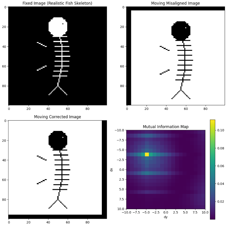
fig, axs = plt.subplots(2, 2, figsize=(10,10))

axs[0,0].imshow(fixed, cmap='gray')
axs[0,0].set_title('Fixed Image (Realistic Fish Skeleton)')

axs[0,1].imshow(moving_misaligned, cmap='gray')
axs[0,1].set_title('Moving Misaligned Image')

axs[1,0].imshow(moving_corrected, cmap='gray')
axs[1,0].set_title('Moving Corrected Image')

cax = axs[1,1].imshow(mi_matrix, extent=[dy_range[0], dy_range[-1], dx_range[-1], dx_range[0]], cmap='viridis')
axs[1,1].set_title('Mutual Information Map')
axs[1,1].set_xlabel('dy')
axs[1,1].set_ylabel('dx')
fig.colorbar(cax, ax=axs[1,1])

plt.tight_layout()
plt.show()

Boundary-based registration

(Greve and Fischl 2009)

Currently considered best for its purpose and is implemented in fMRIprep. Requires surface reconstruction of the anatomical scan.

Coregistration result

# gambling:
file:///home/jovyan/gambling/bids/derivatives/fmriprep/sub-001.html

Corgistration before vs. after

# gambling:
ml freesurfer
freeview \
/home/jovyan/gambling/bids/sub-001/ses-1/anat/sub-001_ses-1_acq-mprage_T1w.nii.gz \
/home/jovyan/gambling/bids/sub-001/ses-1/func/sub-001_ses-1_task-gambling_acq-Fs2_run-1_bold.nii.gz \
/home/jovyan/gambling/bids/derivatives/fmriprep/sub-001/ses-1/func/sub-001_ses-1_task-gambling_acq-Fs2_run-1_space-T1w_desc-preproc_bold.nii.gz

Normalization to template space

Image source: https://publicdomainreview.org/collection/phrenology-diagrams-from-vaught-s-practical-character-reader-1902/

Finally, if you are preforming a group study, you also need to map each individual subject into some common space. This is not a trivial task. As head shpaes of people are different, there brain shapes are also different. Here I tried to draw the approximate shape if each of these guy’s brains, and some hypothetical template brain.

Normalization is needed to compensate for individual differences in brain shape for the group analysis.

Talairach atlas

Image source: Talairach and Tourneux, 1988 (to be confirmed)

Normalization is also needed for a unified coordinate system. You will see that standard coordinates are reported in the articles.

MNI tamplate

Image source:

https://www.bic.mni.mcgill.ca/ServicesAtlases/ICBM152NLin2009

Further reading: https://imaging.mrc-cbu.cam.ac.uk/imaging/MniTalairach

Mapping to template

To match each of them to the template, it is not enough to coregister them as we did for motion correction, because obviously they are of different sizes. We can add 6 more paraeters to the transform, which compensates does scaling and shearing, to better align them. However, there will still be places wehere they do not align perfectly, because one guy one has a bigger frontal lobe, and gy to a bigger parietal lobe

Nonlinear transform

So some software packages use a nonlinear warping algorithm to align brains. There you have to estimate a 3D deformation field and then nonlinearly warp each brain onto a template. They are called non-linear, because different parts of the volume are scaled differently.

Normalization is done using a structural scan

The mapping to common space is usually done via an anatomical scan. First, each subject functional and anatomical scans are coregistered with each other, and then each subject’s anatomical scan is mapped into a template. This is done because the anatomical scan has better quality, and hence the estimated transform is more precise. After you have done that each area in one subject corresponds to the same area in the other subject and you can perform averaging on them.

Volume-based normalization

Unified segmentation

(Ashburner and Friston 2005)

Unified segmentation is still the best algorithm. It performs bias correction, tissue segmentation and normalization in one step.

Surface-based registration

Fsaverage: 40 subjects; Align 39 subjects to 1; create an atlas; align 40 subjects to an atlas; re-create atlas; align 40 subject to the atlas; re-create atlas.

Using knolwdge from freesurfer recon, each voxel together with it’s time course is maped to one of the 3 atlas spaces: either the left cortical hemisphere, the right hemisphere or the subcrotical structures like the basal ganglia, amygldala, brainstem, etc. And the atlas spaces in this case are fsaverage. After this, the spatial smoothing is done either in 2D or in 3D depending on whether it is a surface space or a volume subcortical space, and voxels that do not belong to the space is being basked out.

Spatial smoothing

Finally, each volume is typically smoothed with a gaussian to increase the signal and supress noise. The amount of smoothing is usally expressed by the shape of the gaussian, which, in turn, is described by it’s full withd at half maximum. Here are the examples of the original volume, the smoothed volume at 5 fwhm and 10 fwhm. You can see that the signal increase happens at the expense of the spatial resolution.

Full width at half maximum

Code

# Load library
library(ggplot2)

# Define Gaussian function
gaussian <- function(x, mu = 0, sigma = 1) {
  (1 / (sigma * sqrt(2 * pi))) * exp(- (x - mu)^2 / (2 * sigma^2))
}

# Create data
x <- seq(-5, 5, length.out = 1000)
y <- gaussian(x, mu = 0, sigma = 1)

# Find half maximum
ymax <- max(y)
half_max <- ymax / 2

# Solve for FWHM points
left_idx <- which(y >= half_max)[1]
right_idx <- tail(which(y >= half_max), 1)

x_left <- x[left_idx]
x_right <- x[right_idx]
fwhm_value <- x_right - x_left

# Create data frame
data <- data.frame(x = x, y = y)

# Plot
ggplot(data, aes(x, y)) +
  geom_line(color = "blue", size = 1) +
  geom_hline(yintercept = half_max, linetype = "dashed", color = "red") +
  geom_vline(xintercept = c(x_left, x_right), linetype = "dotted", color = "darkgreen") +
  annotate("text", x = 0, y = half_max + 0.02, label = "Half Maximum", color = "red") +
  annotate("text", x = x_left - 0.3, y = 0.1, label = sprintf("%.2f", x_left), color = "darkgreen") +
  annotate("text", x = x_right + 0.3, y = 0.1, label = sprintf("%.2f", x_right), color = "darkgreen") +
  annotate("text", x = 0, y = 0.15, label = paste("FWHM =", round(fwhm_value, 2)), color = "black", size = 5) +
  theme_minimal() +
  labs(title = "Gaussian Curve with FWHM",
       x = "x",
       y = "Amplitude")

Warning: Using `size` aesthetic for lines was deprecated in ggplot2 3.4.0.
ℹ Please use `linewidth` instead.

Spatial smoothing

Purpose1: increase the signal and suppress the noise

Purpose2: even better compensate for inter-individual differences

FMRIprep does not smooth the data

Critique

(Stelzer et al. 2014)

Volume smoothing has been heavily criticized by some influential people in the field. It has even been called “deficient approaches to human neuroimaging”. Because it does not only degrade the resolution, but also decreases the effect size. But it is still being done in many cases – it all depends on the questions you are asking

Surface-based smoothing

slide courtesy of Doug Greve

5 mm apart in 3D

25 mm apart on surface

Averaging with other tissue types (WM, CSF)

Averaging with other functional areas

One important feature is that fsfast allows surface-based processing, and therefore overcomes some of the difficulties caused by smoothing.

Here is an example of how it works. Here is a piece of freesrurfer reconstructed cortical surface with yellow a white matter surface and red the the gray matter surface. The two points, on opposite banks of the sulcus, are only 5 mm apart in the volume, however, they are very far from each other on the surface. So these two points can be two completely different functional areas. However, if you smooth on the volume, as shown here, you will mix them together. Surface smoothing routines use the information from the freesurfer’s surface reconstruction and smoothe the data along the cortical surface. This allows to take advantage of smoothing procedure without mixing these two areas together.

fMRIprep

Pros

Useful for processing many subjects, whole-brain data, standard acquisition protocols
Collection of best practices from all software
HPC compatibility
Useful for “users” when knowledgeable people assist them
Automatic quality control
Increases reproducibility (?)

Cons

Difficult/impossible to use for custom acquisitions
Difficult/impossible to manually intervene
May not be worth it with few subjects are being processed
Requires a Linux environment and corresponding knowledge
Need integration with the software you will use for your analysis
Hard to explain what you did (black box)

Example I

(Arsenovic, Ischebeck, and Zaretskaya 2022)

Example II

(Coates et al. 2024)

Run fMRIprep

Before running

Apply for a freesurfer license file with your Uni Graz email address: https://surfer.nmr.mgh.harvard.edu/registration.html
Download it and store in /home/jovyan/license.txt (or wherever you like, but make sure you adapt the path in the fMRIprep command below)

Start fMRIprep from neurodesktop

Terminal window

# create freesurfer subject directory
mkdir -p /home/jovyan/gambling/bids/derivatives/fmriprep/sourcedata/freesurfer/

# define the path to the freesurfer subject directory
SUBJECTS_DIR=/home/jovyan/gambling/bids/derivatives/fmriprep/sourcedata/freesurfer/

# run fMRIprep with 4 output spaces: T1 native, MNI, fsnative, fsaverage
fmriprep /home/jovyan/gambling/bids/ /home/jovyan/gambling/bids/derivatives/fmriprep/ \
participant \
--fs-license-file /home/jovyan/license.txt \
--output-spaces T1w MNI152NLin2009cAsym fsnative fsaverage

After this, fMRIprep will run for 4 hours. You do not need to wait for 4 hours! Close neurodesktop and log out. fMRIprep will run in the background. When you come back the next day, everything should be as you left it, with fMRIprep being done. Inspect the html output and submit a screenshot to moodle.

Output spaces

``` {{bash}}
cd /home/jovyan/gambling/bids/derivatives/fmriprep/sub-001/ses-1/func/
ls -l *_bold.nii.gz
```

``` {{bash}}
cd /home/jovyan/gambling/bids/derivatives/fmriprep/sub-001/ses-1/func/
ls -l *_bold.func.gii
```

HTML report

file:///home/jovyan/gambling/bids/derivatives/fmriprep/sub-001.html

Boilerplate

References

Arsenovic, Ana, Anja Ischebeck, and Natalia Zaretskaya. 2022. “Dissociation Between Attention-Dependent and Spatially Specific Illusory Shape Responses Within the Topographic Areas of the Posterior Parietal Cortex.” The Journal of Neuroscience, September. https://doi.org/10.1523/JNEUROSCI.0723-22.2022.

Ashburner, John, and Karl J Friston. 2005. “Unified Segmentation.” NeuroImage 26 (3): 839–51. https://doi.org/10.1016/j.neuroimage.2005.02.018.

Coates, Adam, David Linhardt, Christian Windischberger, Anja Ischebeck, and Natalia Zaretskaya. 2024. “High-Resolution 7T fMRI Reveals the Visual Zone of the Human Claustrum.” Imaging Neuroscience 2 (October): 1–15. https://doi.org/10.1162/imag_a_00327.

Esteban, Oscar, Christopher J. Markiewicz, Ross W. Blair, Craig A. Moodie, A. Ilkay Isik, Asier Erramuzpe, James D. Kent, et al. 2018. “fMRIPrep: A Robust Preprocessing Pipeline for Functional MRI.” Nature Methods 16 (1): 111–16. https://doi.org/10.1038/s41592-018-0235-4.

Greve, Douglas N., and Bruce Fischl. 2009. “Accurate and Robust Brain Image Alignment Using Boundary-Based Registration.” NeuroImage 48 (1): 63–72. https://doi.org/10.1016/j.neuroimage.2009.06.060.

Stelzer, Johannes, Gabriele Lohmann, Karsten Mueller, Tilo Buschmann, and Robert Turner. 2014. “Deficient Approaches to Human Neuroimaging.” Frontiers in Human Neuroscience 8 (July). https://doi.org/10.3389/fnhum.2014.00462.

Tierney, Tim M., Nicholas A. Alexander, Nicole Labra Avila, Yael Balbastre, Gareth Barnes, Yulia Bezsudnova, Mikael Brudfors, et al. 2025. “SPM 25: Open Source Neuroimaging Analysis Software.” https://doi.org/10.48550/ARXIV.2501.12081.