1 Introduction to fMRI
fMRI is a method that allows to non-invasively measure brain activity.
fMRI study examples
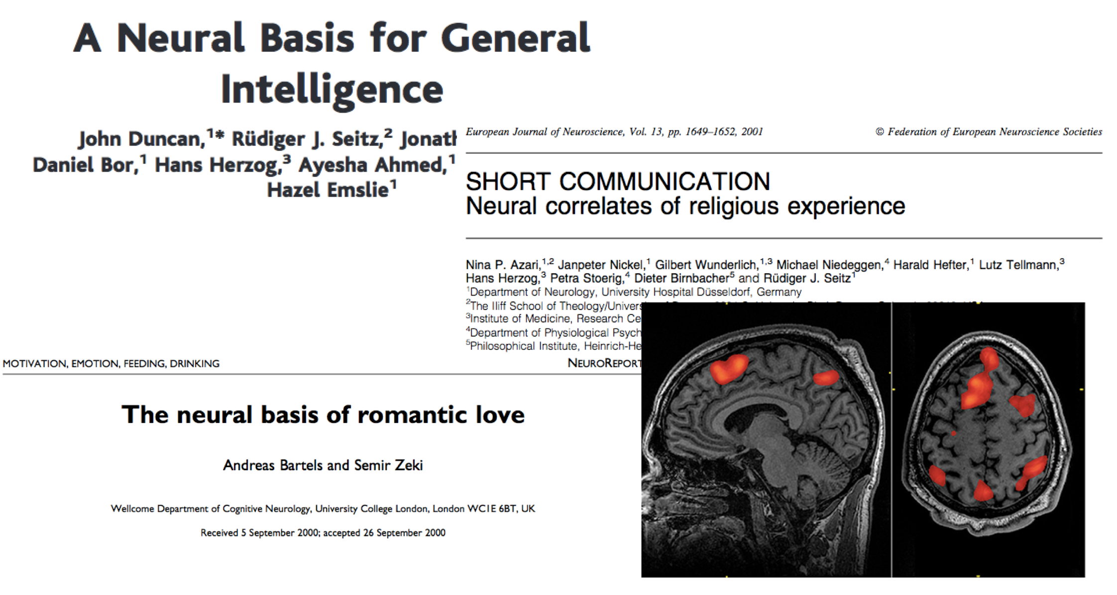
Many crazy studies have been performed with fMRI. Not all of the research questions really make sense!
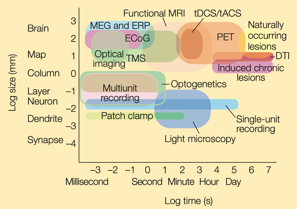
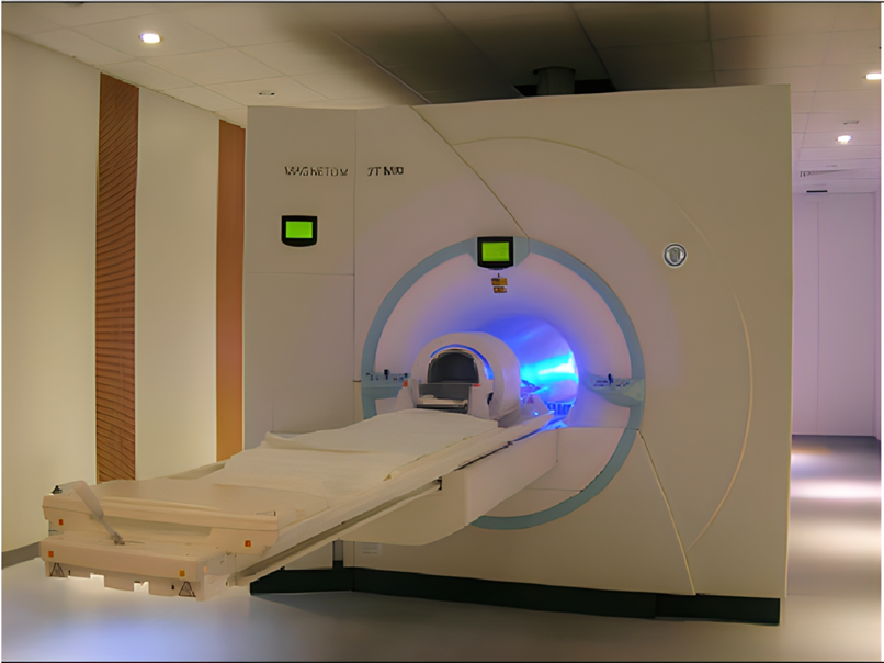
fMRI in comparison
MRI scanner: 3 Tesla
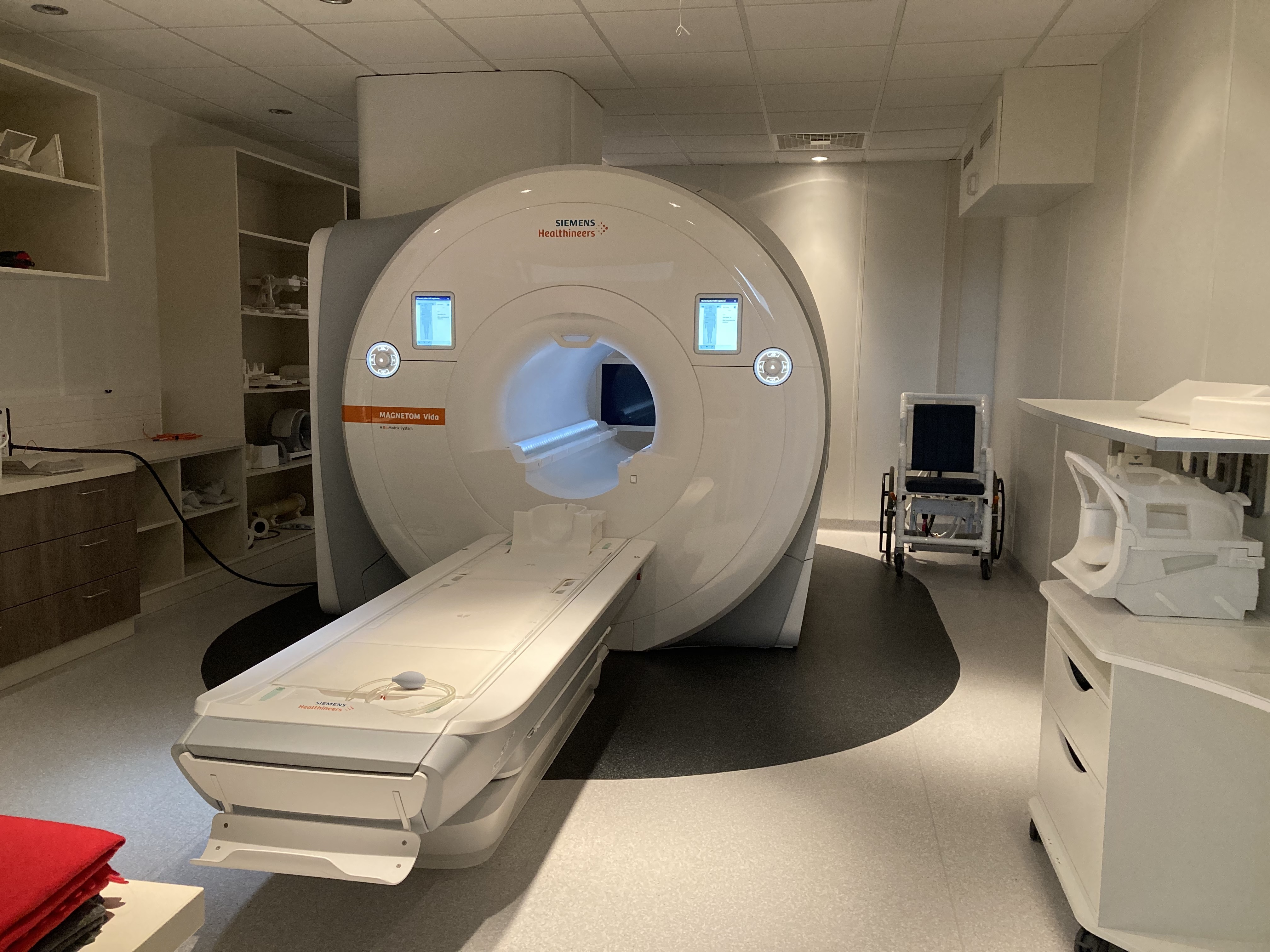
MRI scanner: 7 Tesla
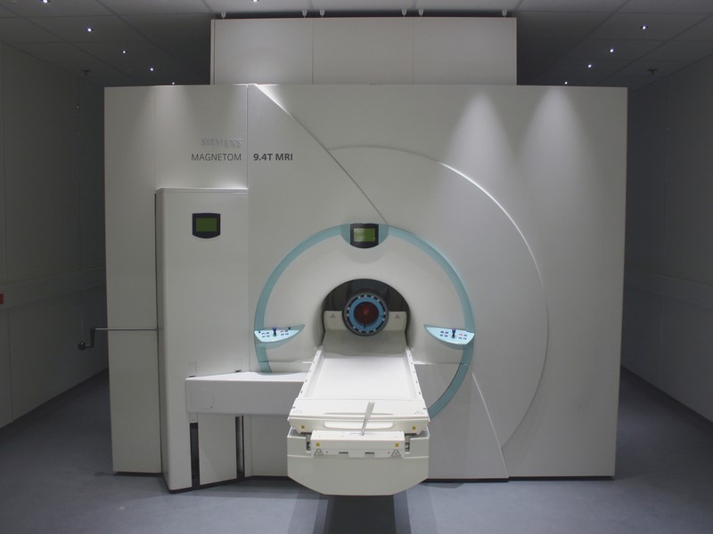
MRI scanner: 9.4 Tesla
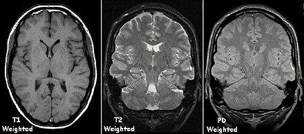
Types of MRI contrasts at 3T
T1w in cognitive neuroscience
Displaying activity on a high-resolution anatomical scan
Quantitative morphometry
Aging
Neurodegeneration
Plasticity
The principle of fMRI
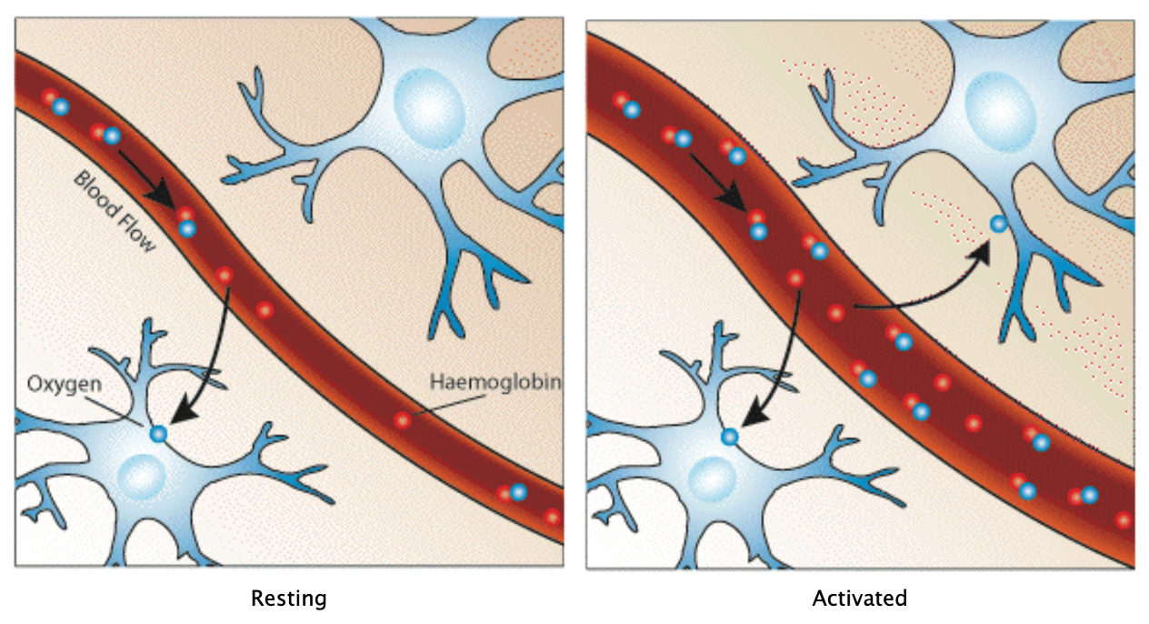
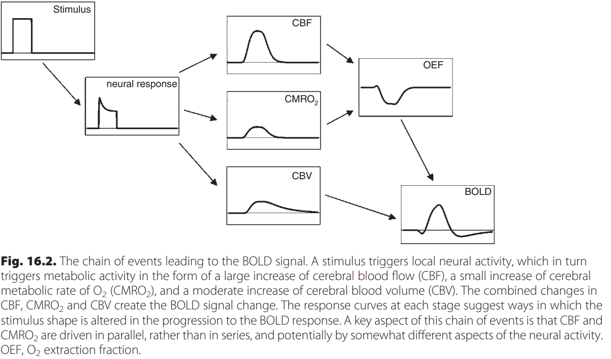
Hemodynamic changes: - increase in blood flow - increase in blood volume - increase in tissue CMRO_2
Hemodynamic response
BOLD signal
blood-oxygen-level-dependent signal
T2*-weighted contrast
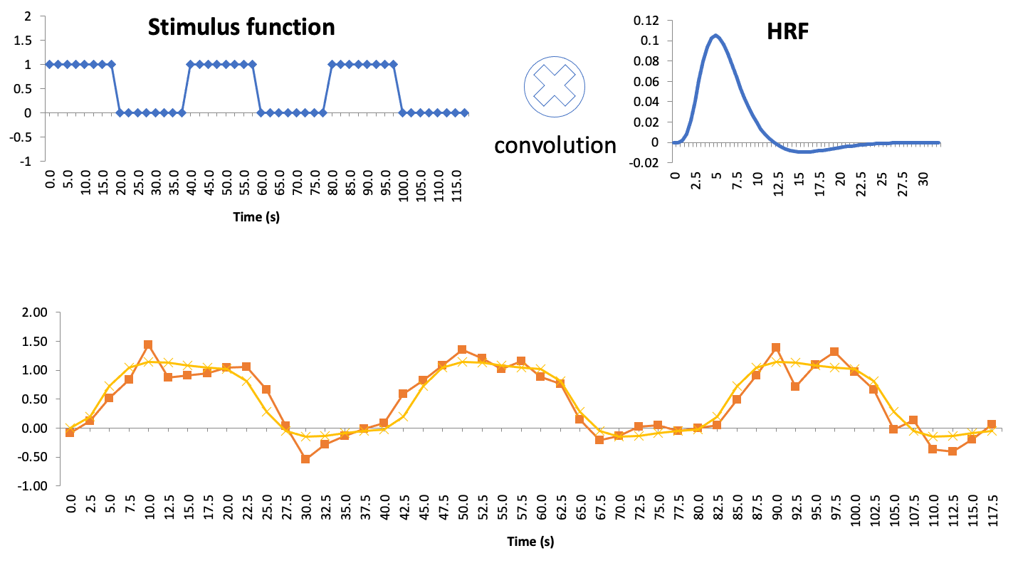
Hemodynamic response function
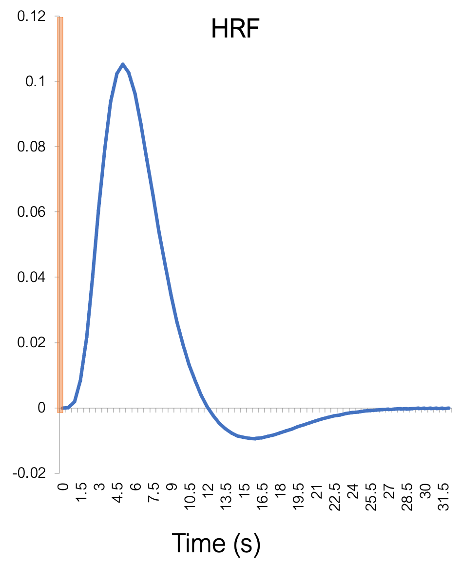
This curve describes the measured signal in response to a brief stimulus.
The response is heavily delayed, and has a relatively complex temporal structure, described by the so called hemodynamic response function (HRF).
After just a brief stimulus that lasts less than a second, the response lasts for seconds. It has a delayed rise phase, a peak, and a subsequent undershoot. The fact that the response is so slow is the main constraint of the temporal resolution of fMRI. It constrains the kind of questions you can ask in your experiment and also puts some constraints on your experimental design.
Neural activity and BOLD
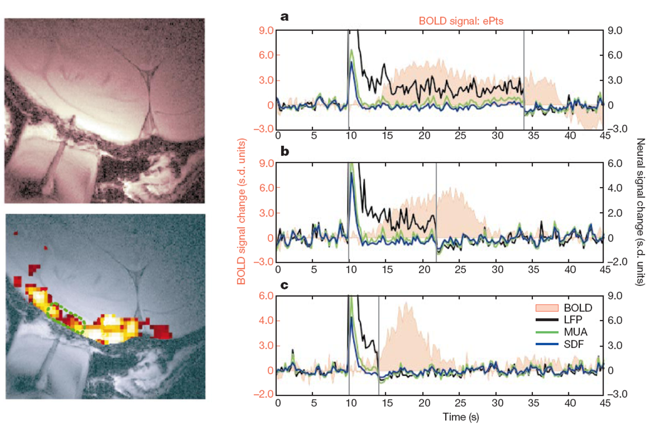
LFP = Local Field Potentials (dendritic currents)
MUA = Multiunit Activity (action potentials)
SDF = Spike-density function (action potentials)
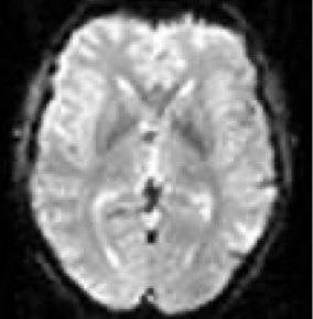
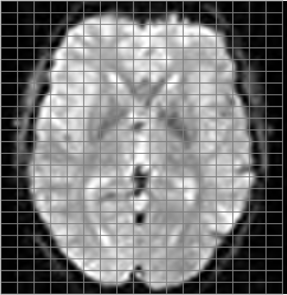
Image acquisition
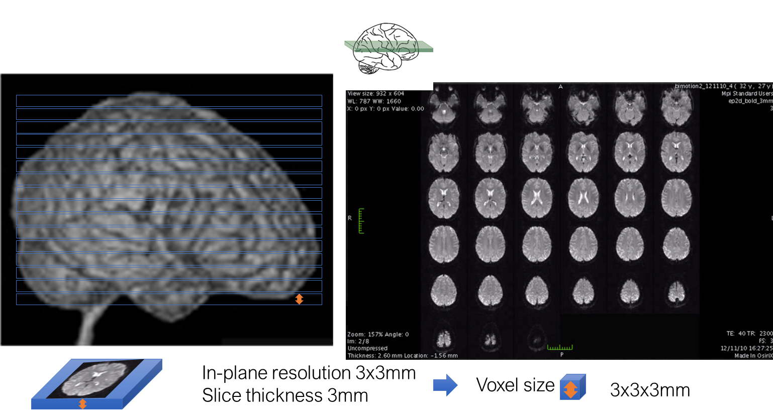
The functional volume is usually acquired slice-by-slice; this is why when you are acquiring the data you see an image like this on the monitor. A functional sequence is characterized by the in-plane matrix size and resolution, as well as by the slice thickness.
Experimental design
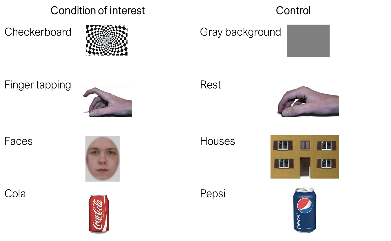
In contrast to e.g. fNIRS, the BOLD-fMRI does not measure the deoxyhemoglobin concentration directly. It is a measure that is weighted by the deoxyhemoglobin concentration, but depends on many other factors like scanner, sequence, participant, and brain area.
This is why any measure of fMRI experiment has to contain at least two conditions, a baseline, and condition of interest. The activation is always computed relative to some baseline. For instance a checkerboard vs gray background, finger tapping versus rest; faces versus houses, etc. And a typical analysis will compare the BOLD signal during condition of interest with rest.
First fMRI experiment
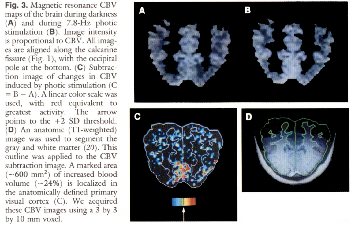
The first experiment was not a BOLD, but a blood volume signal measurement.
First fMRI experiment

This rendering was produced specifically for the cover
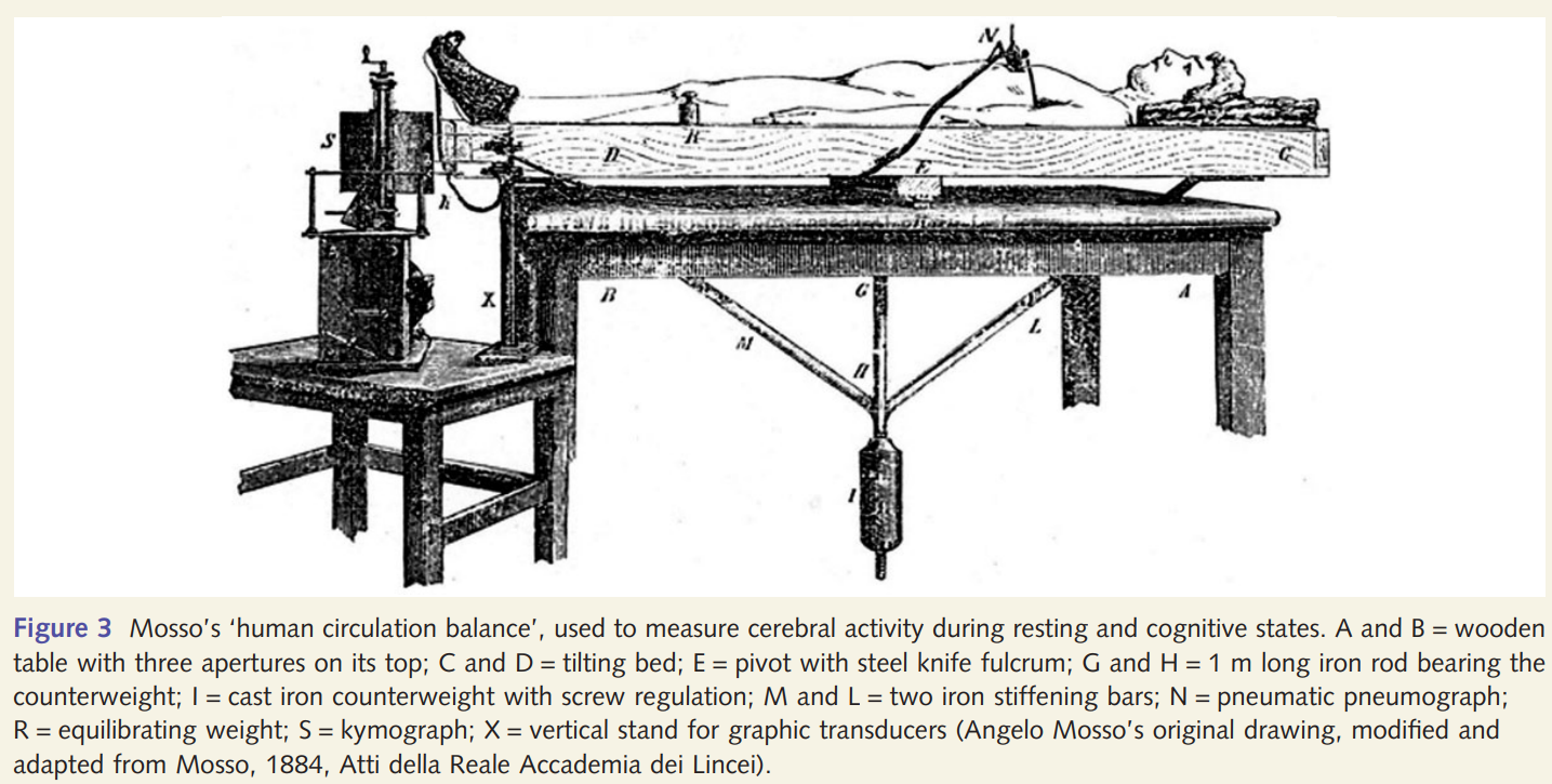
The truly first fMRI experiment
A typical experiment
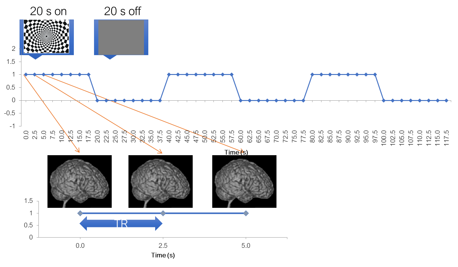
To help us better understand the analysis steps, let’s use an example. Let’s say we have conducted a classical experiment in the visual system, a flickering checkerboard. In this experiment, we want to find out which brain areas are active when subjects view a flickering checkerboard compared to when they view a gray background. We have shown to every volunteer a checkerboard for e.g. 20 second interleaved with a 20 s rest, and we will measure a whole brain volume every 2 seconds, for e.g. to minutes or so.
Matlab code to generate stimulus, BOLD and shifted BOLD X = [1 1 1 1 1 1 1 1 0 0 0 0 0 0 0 0 1 1 1 1 1 1 1 1 0 0 0 0 0 0 0 0 1 1 1 1 1 1 1 1 0 0 0 0 0 0 0 0]; bf = spm_get_bf; % indicated a tr of 2.5 Y = conv(X,bf.bf); Ye = Y+randn(size(Y)).*0.2;
4D dataset
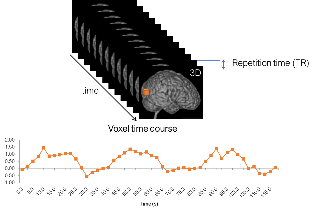
In a functional experiment we usually measure brain activity across the whole volume over extended periods of time, so it is comfortable to think about each functional dataset that we acquire as a 4D dataset, which consists of 3D brain volumes and time as a 4th dimension. This is how the data is typically stored.
A further important parameter is the repetition time (TR). It is the time passes between the acquisition times of two adjacent volumes.
Preprocessing
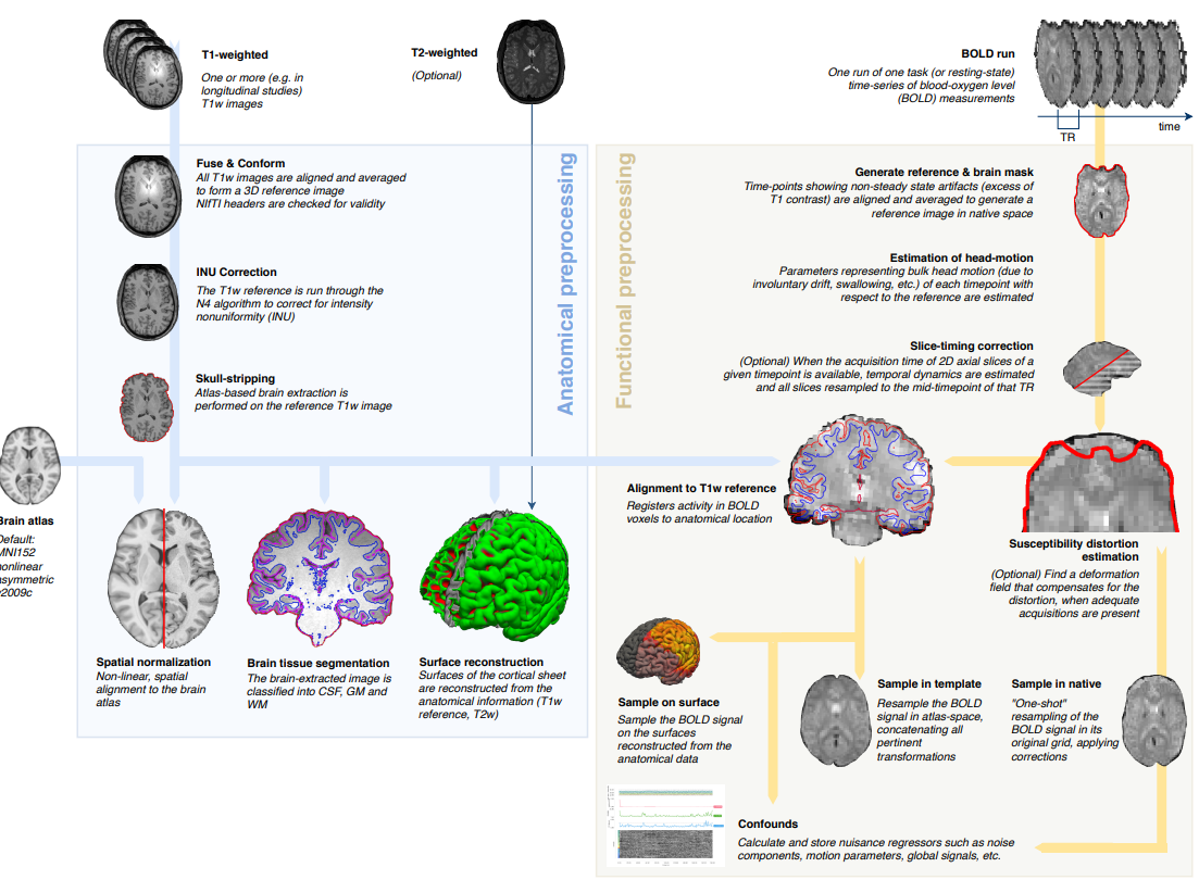
The data quality of modern scanners is typically good enough to skip this step, if your subject is compliant. But it is nevertheless very much advisable and is ALWAYS performed. We will therefore dedicate a whole session to preprocessing. See course schedule for the date.
Analysis steps
Single-subject - first level - fixed effects analysis (FFX)
Group - second-level - random effects analysis (RFX)
(also mixed effects analysis is possible, but relatively rare due to large matrix size)
This is equivalent to e.g. conducting many trials per subject to measure reaction time, and then compute a subject-specific mean per condition, after which you would perform the actual statistical inference
Multilevel modelling is also possible (for small datasets), but less frequent.
Single-subject (first-level) analysis
Univariate/voxel-wise analysis
Question: Which areas are activated by the flickering checkerboard?
Remember that an image is 4d and consists of little 3D cubes called voxels, with the 4th dimension being time. A classical analysis is done over time for every voxel in the brain independently.
Stimulus function
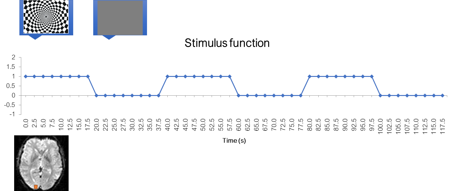
Let’s recall our checkerboard experiment where participants viewed either a checkerboard or a gray screen. Let’s also create a function, called “stimulus function”, which is one where the checkerboard was on, and zero where the checkerboard was off
Side-note on terminology
Trial
Continuous presentation of 1 experimental condition, usually 1-20 seconds
Run
Block of trials separated by interruption of a scanner acquisition, usually 5-10 minutes
Session
Block of runs, separated by subject going out of the scanner and going in again, usually at least one day
Voxel time course
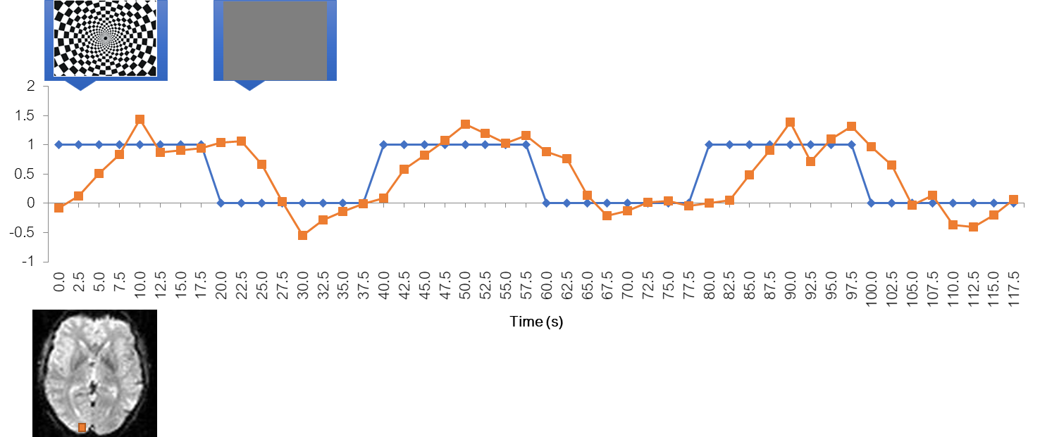
Let’s now look at the time course of a voxel in the visual cortex. You see that it is noisy and delayed, but it kind of follows the stimulus.
Simplest analysis: temporal alignment
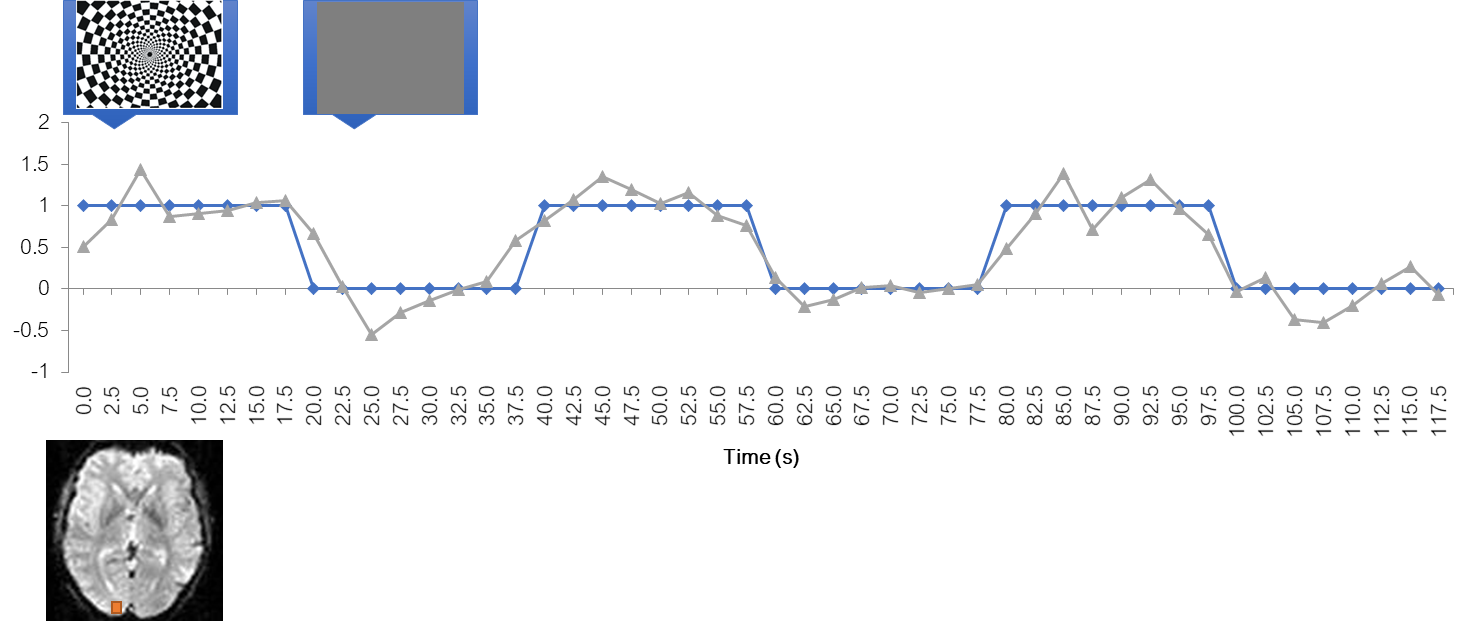
The simplest analysis would be to realign the BOLD time course with the stimulus time course
Simplest analysis: statistical inference
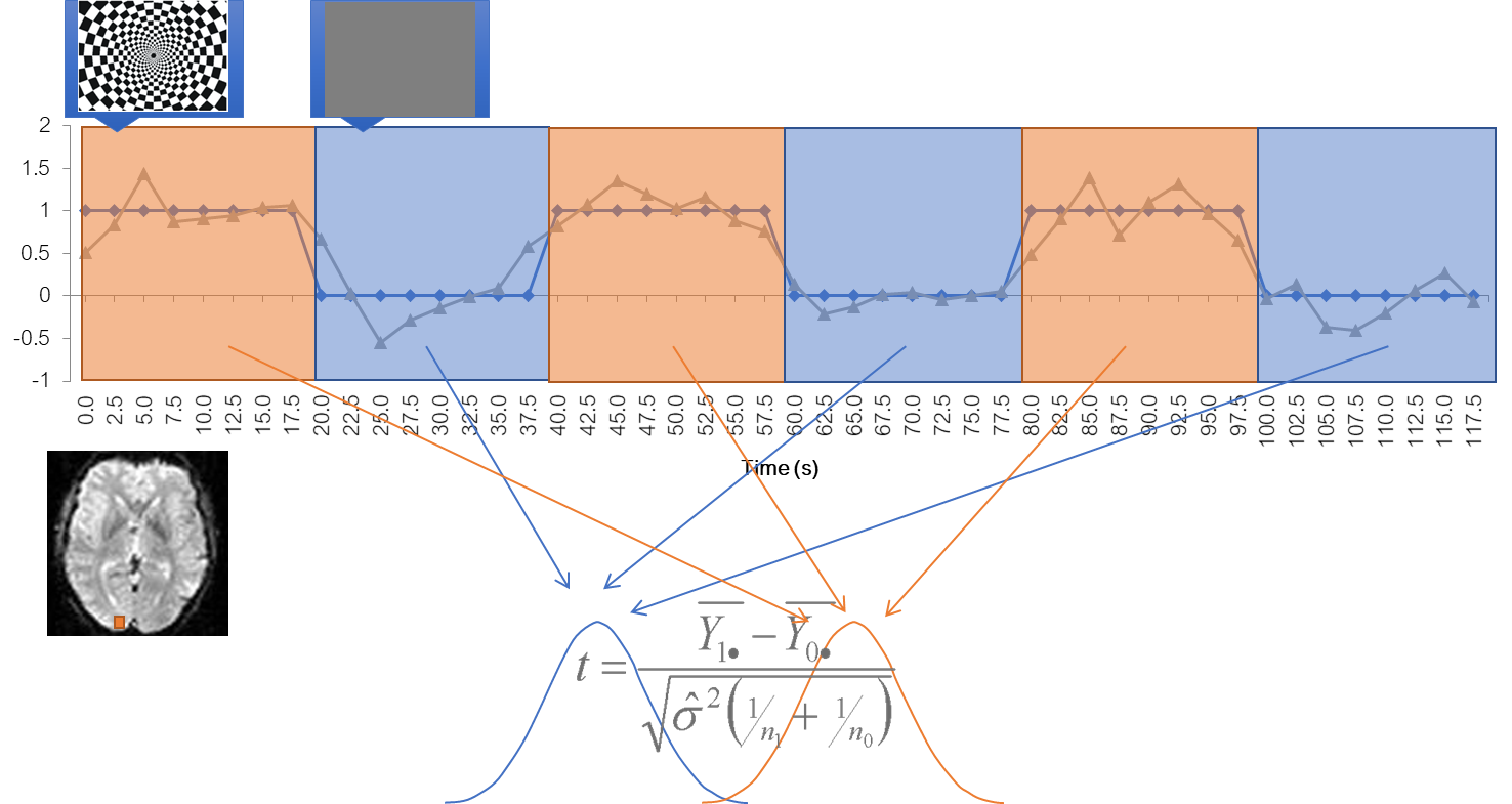
Then label each value according to when it was acquired, stimulus or baseline Collect two types of data points into two big piles and do a statistical comparison via a t-test
Simplest analysis: statistical map
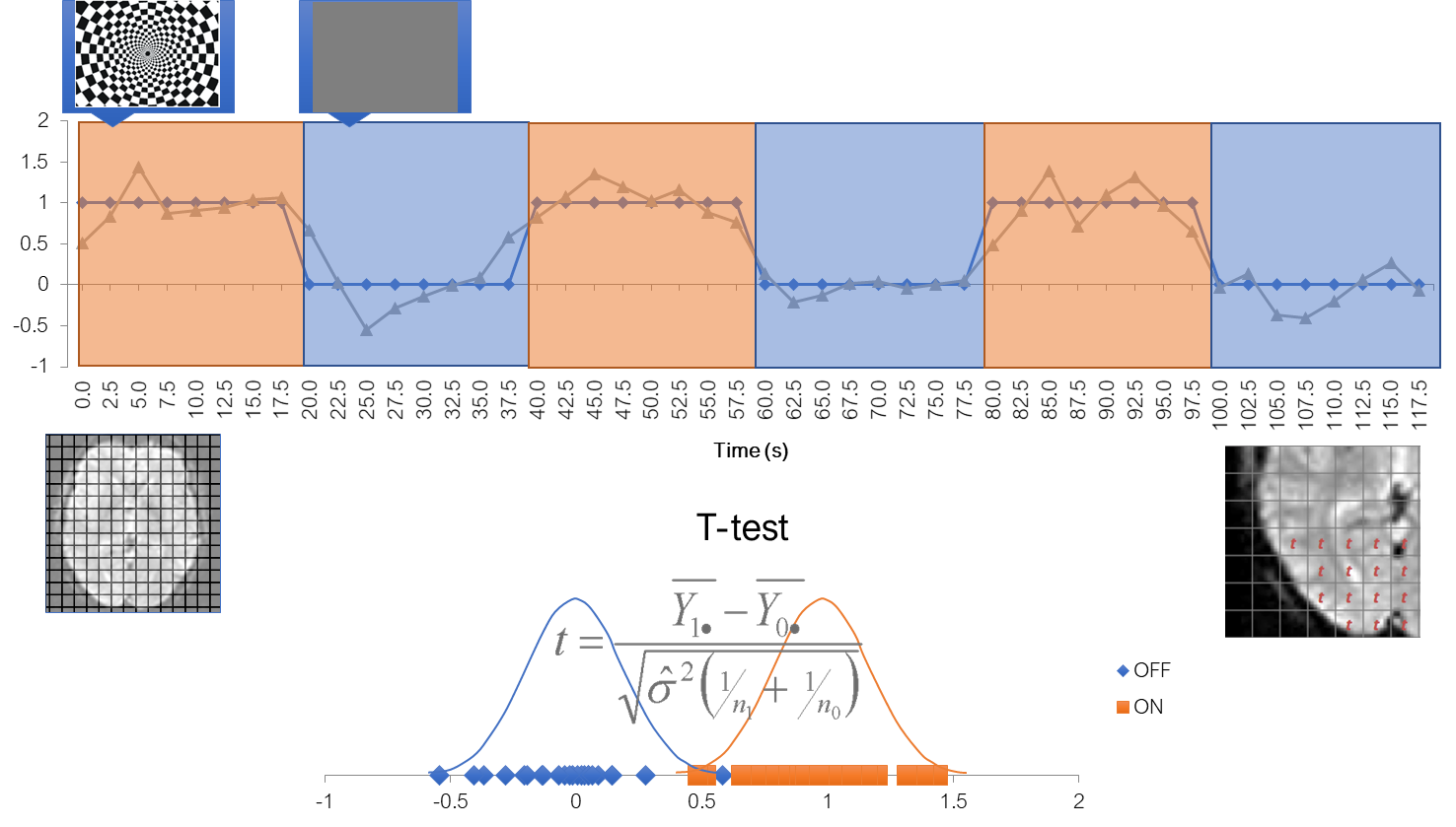
If you do it for every voxel, you can get a new volume, which consists of t-statistics
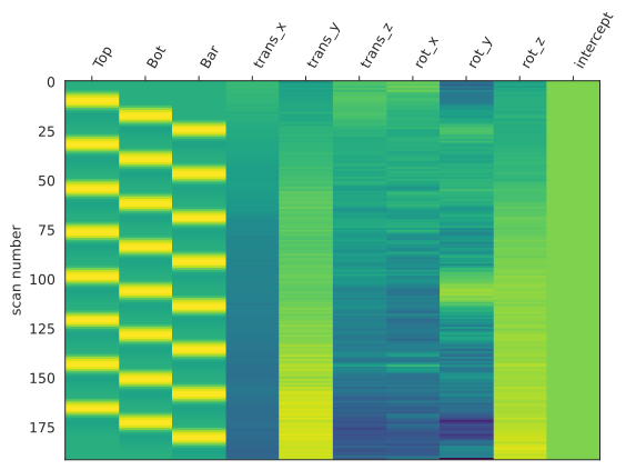
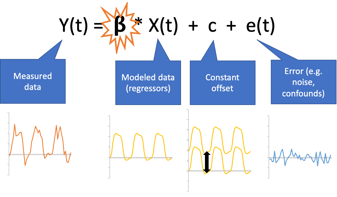
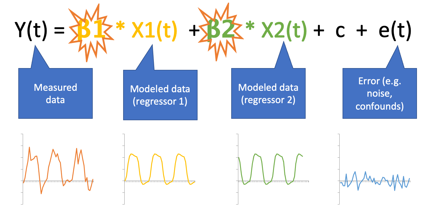
General Linear Model (GLM)
Multiple regression with ingredients:
Predictor(s): stimulus function convolved with the HRF (see Buidling regressors)
Nuissance regressors
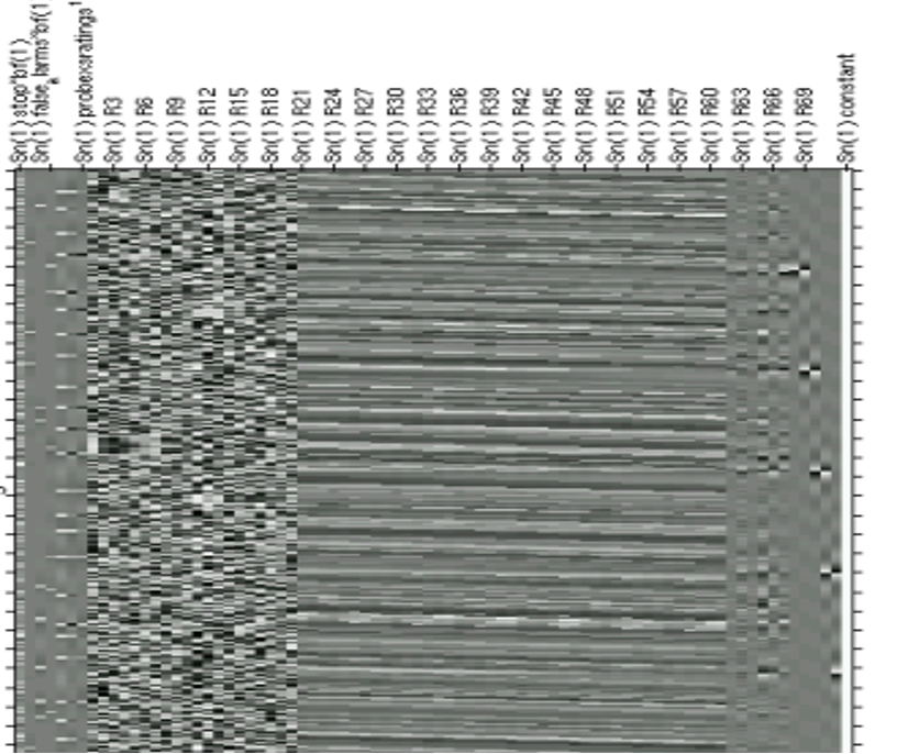
Buidling regressors
General linear model
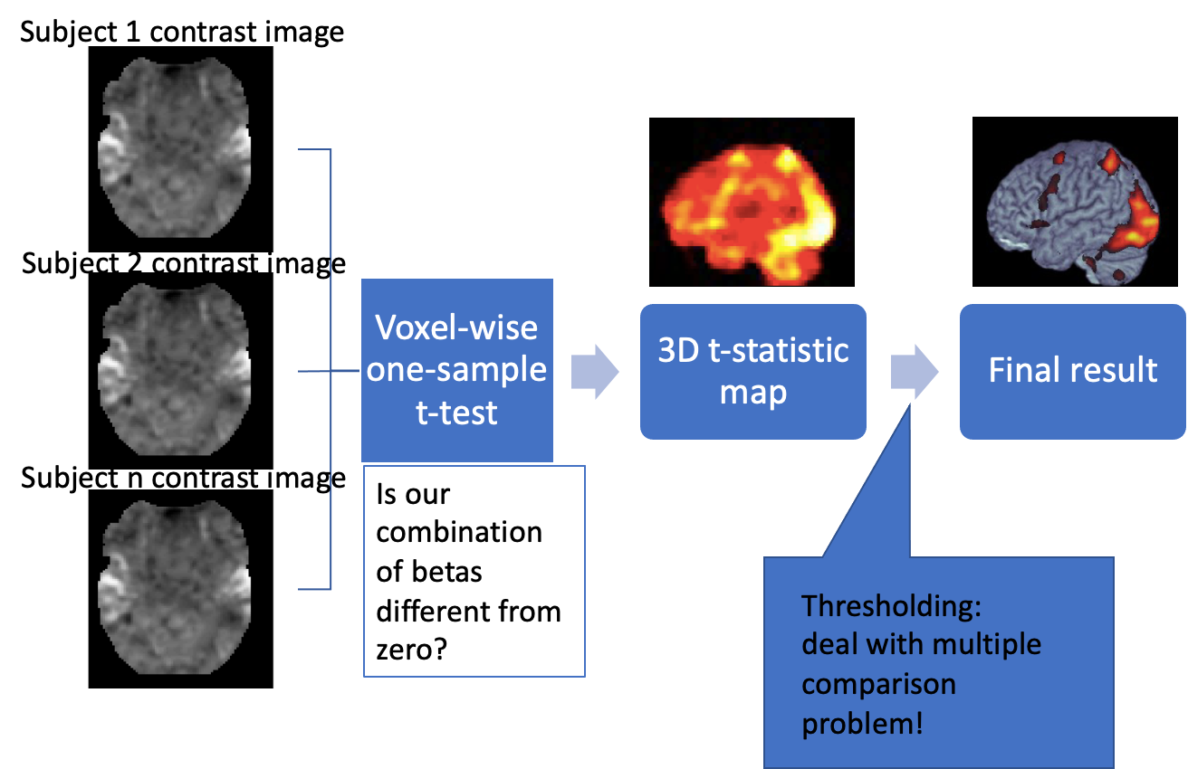
Statistical inference in whole-brain analysis
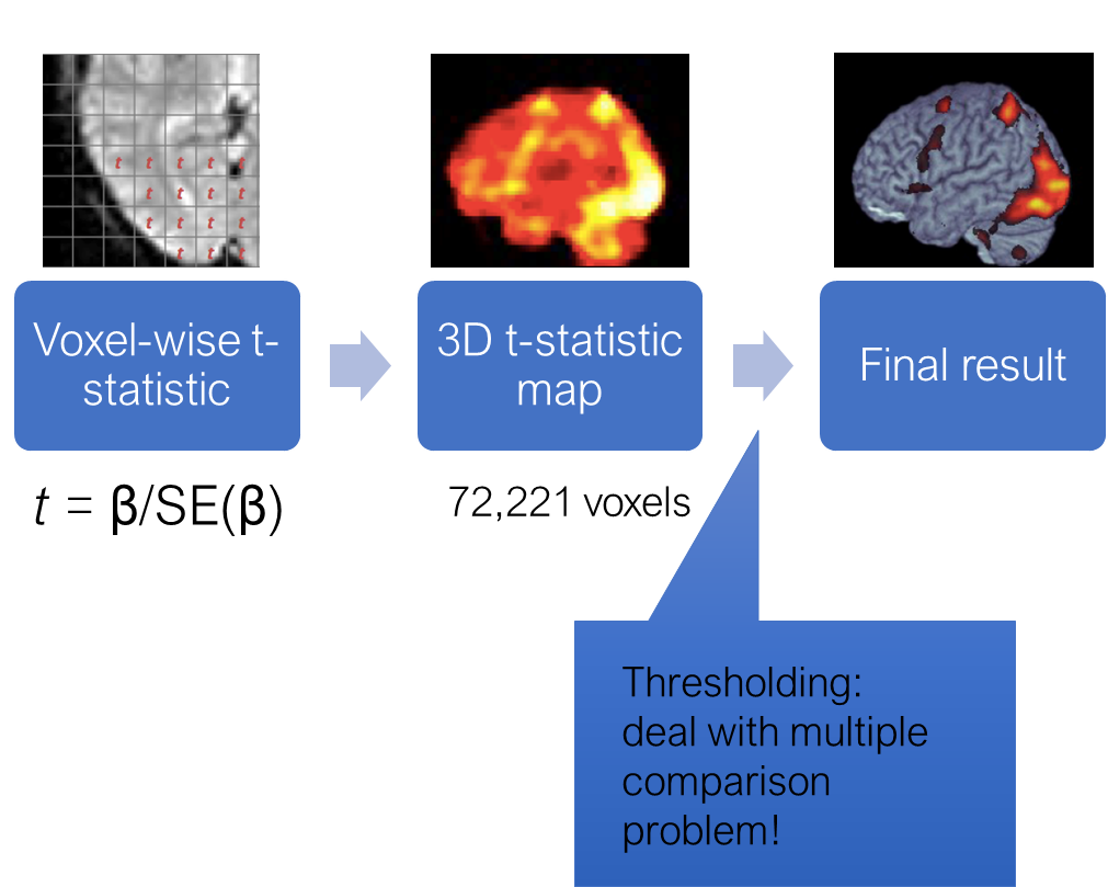
How do we get from beta estimates to making statistical inference? As in a typical regression, beta estimate divided by its standard error is a t-statistic with a t-distribution. So to know whether an activation in one voxel is significant is relatively straightforward.
If we had just one voxel, we would have computed the t-statistic, and then depending on the degrees of freedom determined if it exceeds the critical value. However, we are doing the same statistical test for MANY voxels. SO the probability that we find a significant voxel simply by chance increases. This is the multiple comparison problem that is encountered anywhere in statistics. In fMRI it is particularly prominent, because the number if singe tests is enormous. There are several ways and philosophies for dealing with it, I won’t go into details right now. The important thing is that any voxel-wise analysis MUST deal with this problem in some way.
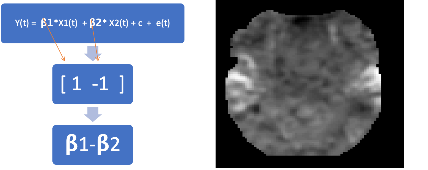
Two conditions
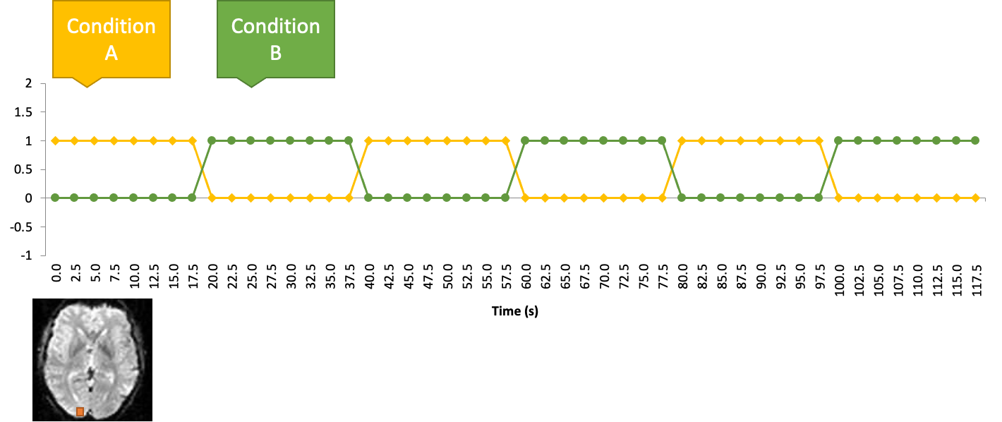
General linear model with two conditions
Contrast
A linear combination of beta estimates
GLM advantages
Complex experimental designs
Discounting uninteresting effects/confounds
HRF shape estimation
Group analysis
Region-of-interest (ROI) analysis
Question: Does the primary visual cortex respond to flickering checkerboards?
ROI analysis is a way to deal with multiple comparison problem. But it requires an a priory and independent definition of an ROI.
There are two ways to define ROIs:
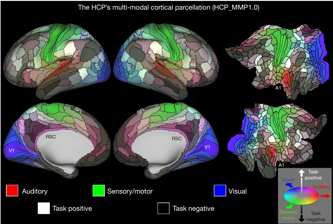
From an anatomical scan
From an additional (separate) functional experiment
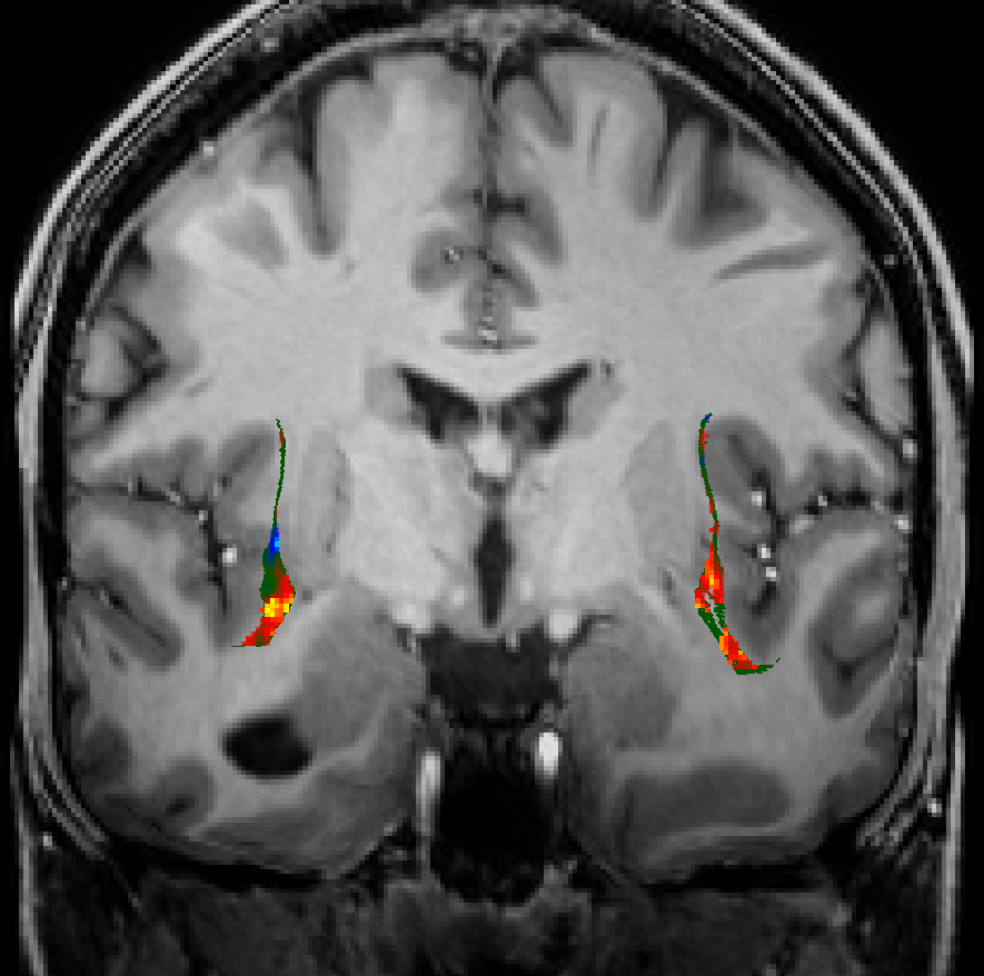
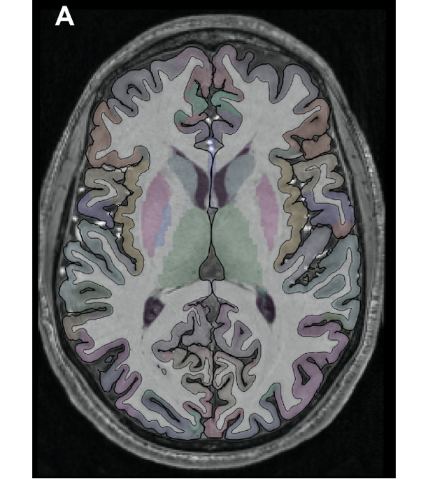
Subcortical ROIs
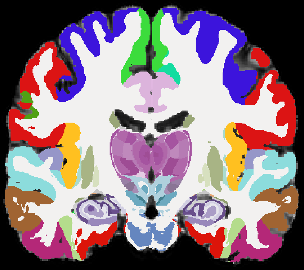
This is the state-of-the-art for anatomically-based ROI definition based on deep learning